新しいタスクの作成
ダウンロード
フォーカスモード
フォントサイズ
このドキュメントでは、定时SQL分析タスクを新規作成する方法について説明します。
前提条件
CLSを有効にしており、ソースログトピックでキー値インデックスを有効にしています。
現在の操作アカウントに定时SQL分析を設定する権限があることを確認してください。詳細はCLSアクセスポリシーテンプレートをご参照ください。
操作手順
1. CLSコンソールにログインし、左側のナビゲーションバーで定时SQL分析を選択し、新規作成をクリックします。
2. 定时SQL分析タスクを設定します。このうち書き込み先は指標トピックとログトピックに分けられます。
書き込み先がログトピックの場合:ログフィルタリング、ログ事前集計などのシナリオに使用されます。
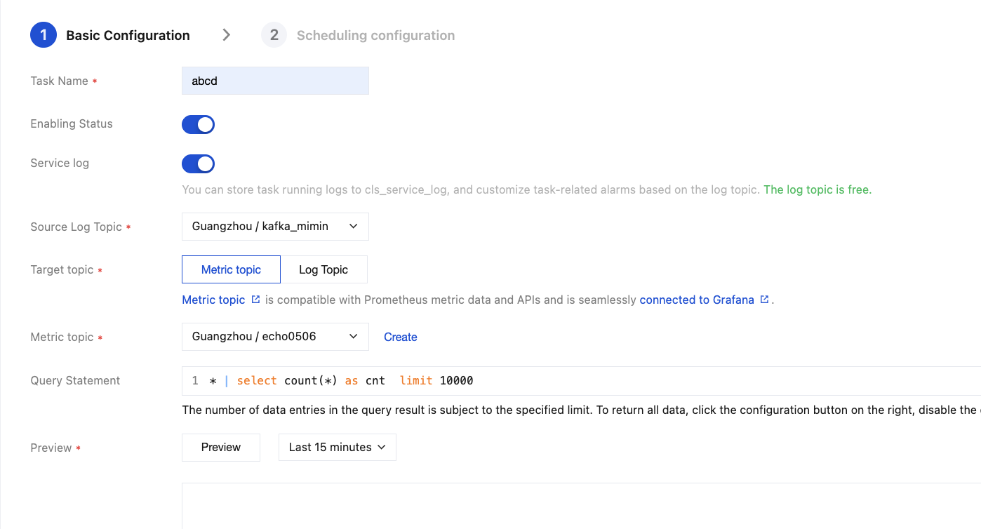
ユースケース:
事前集計です。例えば、ログが10秒ごとに1回報告され、ビジネスで60日分のデータをクエリする必要がある場合:
*| select count(*) group by ip, request_method、IPは60日間で1億件を超える可能性があり、次元が高すぎるためクエリが失敗します。その場合、ログから指標への変換を使用して、ログを分レベルの指標データに事前集計し、その後集計済みの指標トピックをクエリすればタイムアウトしません。指標変換ストレージの利点:
クエリ費用が低い:指標はストレージ料金と書き込みトラフィック料金のみが発生し、インデックストラフィック料金とインデックスストレージ料金は発生しません(ログにはあります)。同じデータ量の場合、指標のクエリ費用はより低くなります。詳細は製品価格をご参照ください。
ストレージ費用:特に長期間の時間範囲をクエリする必要があるビジネスの場合、指標に変換した後、元のログ沈降を低頻度ストレージに移行できます(低頻度はSQLをサポートせず、検索可能です)。これにより、ログストレージ費用をさらに節約できます。
クエリ速度がより高速です。詳細はログから指標への変換をご参照ください。
設定項目:
設定項目 | 説明 |
タスク名 | スケジュールSQLタスクの名前です。長さは255文字で、アンダースコア、英字、数字の組み合わせです。 |
有効状態 | デフォルトでは有効です。タスクを有効/無効にします。 |
サービスログ | 有効/無効です。有効にすると、定時SQLタスクの実行監視メトリックがサービスログに書き込まれます。例えば、単一クエリ結果、クエリ時間などです。 |
ソースログトピック | 定時SQLタスクの入力です。つまり、メトリックに変換する必要がある元のログが存在するログトピックです。 |
書き込み先 | メトリックトピック/ログトピック。 |
実行ステートメント | SQLステートメントを使用して生ログを統計処理し、指標を取得します。例: * | select avg(cpu_usage)as cpu_usage ,avg(mem_usage) as mem_usage,namespace,cluster group by namespace,cluster limit 10000説明: SQLステートメントを変更した場合は、プレビューをクリックして、SQLクエリ結果を更新してください。 クエリ結果件数は、指定したlimitに従って返されます。全量データを返す必要がある場合は、実行ステートメント右側の設定ボタンをクリックし、SQL結果デフォルトLimitスイッチをオフにして、実行ステートメント内のlimitを削除してください。 |
指標名 | 複数選択可能で、通常は数値タイプです。ドロップダウンリストから指標名としてフィールドを選択します。例えば、上記の例では、cpu_usageとmem_usageが指標名であり、その値が指標値です。 |
指標ディメンション | 複数選択可能です。選択できない時間型フィールドは指標ディメンションとして使用できません。ドロップダウンリストから指標ディメンションとしてフィールドを選択します。例えば、上記の例では、namespace、clusterがディメンションであり、その値がディメンション値です。異なるclusterとnamespaceの組み合わせに基づいてcpu_usageとmem_usageを確認すると理解できます。指標ディメンションは通常、SQLステートメント内のgroup byのディメンションフィールドです(時間型フィールドを除く)。 |
カスタムディメンション | 新しい指標のディメンションで、ディメンション値は静的です。例えば:元の指標ディメンションが go_gc_duration_seconds{job="prometheus",quantile="0"}カスタムディメンション tcloud_region_name="ap-guangzhou"を追加すると、ディメンションは次のようになります。go_gc_duration_seconds{job="prometheus", quantile="0",tcloud_region_name="ap-guangzhou" } |
タイムスタンプ | デフォルト値(クエリ時間枠の左側の時刻):指標のデフォルトタイムスタンプはクエリ時間枠の左側の時刻です。例えば、クエリ時間枠が5月7日00:00:00~5月7日00:10:00の場合、この計算で生成される指標タイムスタンプは5月7日00:00:00です。 クエリ時間枠の右側の時刻:指標のデフォルトタイムスタンプはクエリ時間枠の右側の時刻です。例えば、クエリ時間枠が5月7日00:00:00~5月7日00:10:00の場合、この計算で生成される指標タイムスタンプは5月7日00:10:00です。 カスタムタイムスタンプ:SQLステートメントで時間タイプのフィールドをカスタマイズした場合、ドロップダウンリストでそのフィールドを指標のタイムスタンプとして選択できます。その時間タイプのフィールドが表示されない場合は、SQLステートメントの下にあるプレビューをクリックして、ドロップダウンリストのフィールド値を更新してください。 説明: カスタムタイムスタンプは、UNIX時間、TimeStampのタイプを選択できます。精度はミリ秒です。例えば、1629876543.123、2021-08-25T12:22:23.123+08:00です。 |
スケジュール範囲 (Scope) | 定時SQLタスクが処理するログデータの範囲です。例えば、2023年1月1日00:00:00から2023年3月31日00:00:00までのログの場合、終了時間を選択しないと、タスクは継続的に実行され、新しく収集されたログを継続的に指標へ変換します。 |
スケジュール周期 | 分単位と秒単位の2種類の周期タイプをサポートしています。業務の即時性要件に応じて柔軟に選択できます。 分単位:値の範囲は1分~1440分です。例えばXに設定した場合、X分ごとに1回ログクエリが実行され、ログクエリの結果は指標として保存されます。 秒単位:選択可能な値は10秒、15秒、20秒、30秒で、指標データを生成するシーンに適しています。秒単位を選択した後、クエリ時間枠の値の単位は秒をサポートし、ウィンドウサイズの下限は10秒、上限は60秒です。周期内のQuery実行時間が設定したスケジュールウィンドウを超えた場合は、より大きなスケジュール周期を選択することをお勧めします。タスクのスケジュール詳細で確認できます。 |
クエリ時間枠 (Query Window) | スケジュール周期が分単位の場合:@m-1m~@mを設定することをお勧めします。これは直近1分間を意味し、毎回1分間のログデータをクエリして、対象トピックに保存します。 注意: 指標に変換する際、このパラメータは30分を超えないようにしてください。超えた場合、指標への変換が失敗する可能性があります。 クイック設定:近5分間を選択した場合、現在時刻が17:30であれば、クエリ時間枠は17:25~17:30です。 時間式:相対時間の表現に適用されます。例えば、指定した時間式が@m-10m~@m-5mで、現在時刻が17:30の場合、クエリ時間枠は17:20~17:25です。 スケジュール周期が秒単位の場合:@s-15s~@sを設定することをお勧めします。これは直近15秒を意味し、毎回15秒のログデータをクエリして、対象トピックに保存します。 注意: スケジュール周期が秒単位の場合、クエリ時間枠の値の範囲は[10秒, 60秒]です。誤った時間式の例: ウィンドウが10秒未満の場合:@s-9s~@sでは、クエリ時間枠のサイズが9秒しかないため、エラーが発生します。 ウィンドウが60秒を超える場合:@s-61s~@sでは、クエリ時間枠のサイズが61秒となり、ウィンドウの最大値を超えます。 時間を最長1時間遡ることができ、対応する時間式は@s-3600s~@s-3540sです。 クイック設定:近10秒を選択した場合、現在時刻が15:58:00であれば、クエリ時間枠は15:57:50~15:58:00です。 時間式:相対時間の表現に適用されます。例えば、指定した時間式が@s-20s~@s-10sで、現在時刻が15:58:00の場合、クエリ時間枠は15:57:40~15:57:50です。 |
詳細設定 | クエリ遅延時間です。コンソールの詳細設定で、値の範囲は0秒から120秒です。ログのインデックス生成には通常遅延が発生し、インデックス生成前はクエリできません。この時点でインデックスは生成済みです(99.9%のインデックスデータは5秒以内に生成されます)。分単位の遅延実行のデフォルトは60秒で、秒単位クエリの遅延実行のデフォルトは30秒です。 |
ユースケース:
ログフィルタリング:
*| SELECT ip where region="guangzhou" 注意:
タイマーSQLの実行は1分遅延します。例えば、11:01~11:02のデータをクエリする場合、クエリは11:03に開始され、最大100万件のデータが返されます。お客様のシナリオに適合するかどうかを評価する必要があります。
事前集計です。例えば、ログが10秒ごとに1回報告され、ビジネスで60日分のデータをクエリする必要がある場合:
*| SELECT ip , AVG(request_time) AS avg_request_time GROUP BY ip、IPは60日間で1億件を超える可能性があり、次元が高すぎるためクエリが失敗します。その場合、タイマーSQLを使用して秒単位のログを分単位のデータに事前集計し、その後集計済みのデータをクエリすればタイムアウトしません。設定項目:
設定項目 | 説明 |
タスク名 | スケジュールSQLタスクの名前です。長さは255文字で、アンダースコア、英字、数字の組み合わせです。 |
有効状態 | デフォルトでは有効です。タスクを有効/無効にします。 |
サービスログ | 有効/無効です。有効にすると、定時SQLタスクの実行監視メトリックがサービスログに書き込まれます。例えば、単一クエリ結果、クエリ時間などです。 |
ソースログトピック | 定時SQLタスクの入力です。処理対象の元のログです。 |
書き込み先 | 定時SQLタスクの出力(1つ)です。ログトピックを選択し、事前にターゲットトピックのインデックスを設定することをお勧めします。 |
実行ステートメント | SQL文を使用して元のログを統計します。例えば、スケジュール周期を1分に設定し、クエリ時間枠を1時間に設定した場合、SQL文は *| select sum(active_user) as hourly_active_user limit 10000となり、毎分直近1時間のアクティブユーザー数を統計することを表します。説明: SQLステートメントを変更した場合は、プレビューをクリックして、SQLクエリ結果を更新してください。 クエリ結果件数は、指定したlimitに従って返されます。全量データを返す必要がある場合は、実行ステートメント右側の設定ボタンをクリックし、SQL結果デフォルトLimitスイッチをオフにして、実行ステートメント内のlimitを削除してください。 |
タイムスタンプ | デフォルト値(クエリ時間枠の左側の時刻):デフォルトタイムスタンプはクエリ時間枠の左側の時刻です。例えば、クエリ時間枠が5月7日00:00:00~5月7日00:10:00の場合、この計算で生成されるタイムスタンプは5月7日00:00:00です。 クエリ時間枠の右側の時刻:デフォルトタイムスタンプはクエリ時間枠の右側の時刻です。例えば、クエリ時間枠が5月7日00:00:00~5月7日00:10:00の場合、この計算で生成されるタイムスタンプは5月7日00:10:00です。 カスタムタイムスタンプ:SQLステートメントで時間タイプのフィールドをカスタマイズした場合、ドロップダウンリストでそのフィールドをタイムスタンプとして選択できます。その時間タイプのフィールドが表示されない場合は、SQLステートメントの下にあるプレビューをクリックして、ドロップダウンリストのフィールド値を更新してください。 説明: カスタムタイムスタンプは、UNIX時間、TimeStampのタイプを選択できます。精度はミリ秒です。例えば、1629876543.123、2021-08-25T12:22:23.123+08:00です。 |
スケジュール範囲 (Scope) | 定時SQLタスクが処理するログデータの範囲です。例えば、2023年1月1日 00:00:00から2023年3月31日00:00:00までのログの場合、終了時間を指定しないと、デフォルトで継続的に実行されます。 |
スケジュール周期 | 値の範囲は1分~1440分です。1分に設定した場合、1分ごとにログクエリが1回実行されます。 |
クエリ時間枠 (Query Window) | クエリ時間枠です。単一ログクエリの時間枠です。 クイック設定:近5分間を選択した場合、現在時刻が17:30であれば、クエリ時間枠は17:25~17:30です。 時間式:相対時間の表現に適用されます。例えば、指定した時間式が@m-10m~@m-5mで、現在時刻が17:30の場合、クエリ時間枠は17:20~17:25です。 |
詳細設定 | クエリ遅延時間です。コンソールの詳細設定で、値の範囲は0秒から120秒です。ログのインデックス生成には通常遅延が発生し、インデックス生成前はクエリできません。この時点でインデックスは生成済みです(99.9%のインデックスデータは5秒以内に生成されます)。分単位の遅延実行のデフォルトは60秒で、秒単位クエリの遅延実行のデフォルトは30秒です。 |
時間表現の構文
タイマーSQL分析を作成する際に、SQL時間枠を指定できます。タイマーSQLタスクの実行時には、そのSQL時間枠内のログのみをクエリします。以下では、SQL時間枠に関連する時間式の構文について説明します。
演算子 | 説明 |
+ | プラス記号 |
- | マイナス記号 |
@ | 切り捨て演算子は、時間に基づいて切り捨てます。例えば、時間を1時間単位で01:40に切り捨てる場合、切り捨て後は01:00になります。 |
時間単位 | 説明 |
h | 時 |
m | 分 |
s | 秒 |
例
時間式 | 説明 |
@m-15m から @m-5m | 例えば、スケジュールSQLタスクを作成する場合、スケジュール範囲は毎日00:00から開始され、遅延実行は30秒、SQL時間ウィンドウは[@m-15m,@m-5m)です。最初の分析は00:00:30に実行され、[23:45~23:55)の期間のデータを分析します。以降も同様に、周期的にスケジュール分析が行われます。 |
@h-1h から @h | 例えば、スケジュールSQLタスクを作成する場合、スケジュール範囲は毎日00:00から開始され、遅延実行は30秒、SQL時間ウィンドウは[@h-1h,@m-5m)です。最初の分析は00:00:30に実行され、[23:00~23:55)の期間のデータを分析します。以降も同様に、周期的にスケジュール分析が行われます。 |
@s-10s から @s | 例えば、スケジュールSQLタスクを作成する場合、スケジュール範囲は毎日00:00:00から開始され、遅延実行は30秒、SQL時間ウィンドウは[@s-10s,@s)です。最初の分析は00:00:30に実行され、[23:59:50~23:59:00)の期間のデータを分析します。以降も同様に、周期的にスケジュール分析が行われます。 |
@h-12h+5m から @m-5m | 例えば、スケジュールSQLタスクを作成する場合、スケジュール範囲は毎日00:00から開始され、遅延実行は30秒、SQL時間ウィンドウは[@h-12h+5m,@m-5m)です。最初の分析は00:00:30に実行され、[12:05~23:55)の期間のデータを分析します。以降も同様に、周期的にスケジュール分析が行われます。 |
フィードバック